Quick Start Guide: Length Based Spawning Potential Ratio

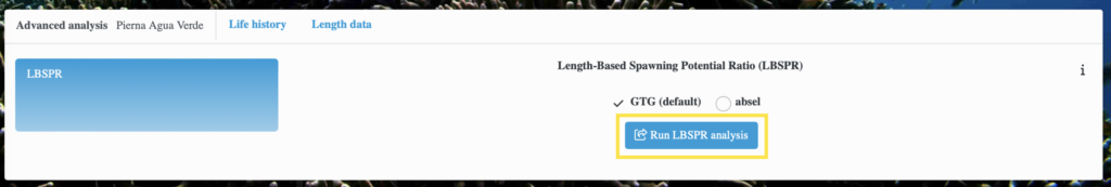
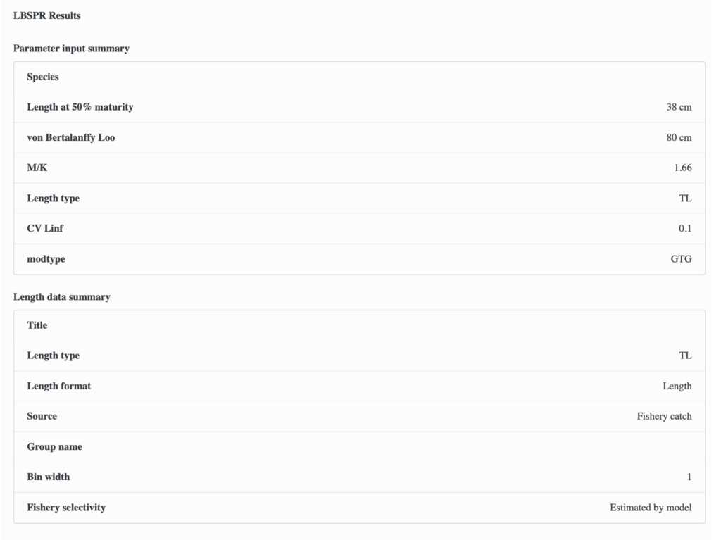
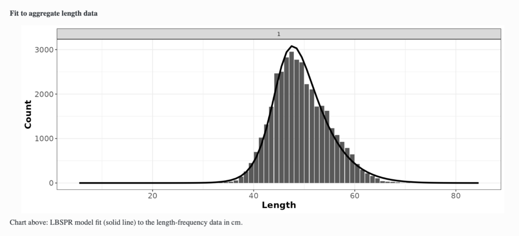
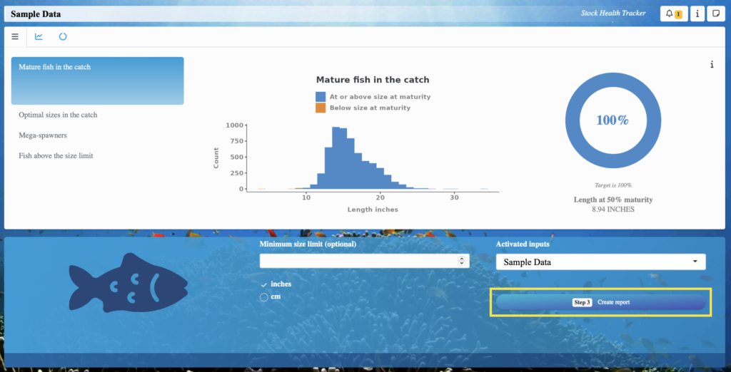
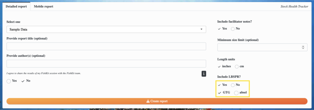
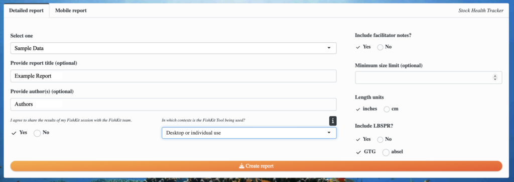
Here we’ll walk through the steps to run a Length-Based Spawning Potential Ratio (LBSPR) analysis within the Stock Health Tracker. LBSPR is a more complex method that can be used to assess stock health, but should be applied and interpreted with care as it is not appropriate for all species or fisheries contexts. An in depth description of this model and its associated assumptions can be found here. We strongly recommend consulting this paper and/or a fisheries scientist before incorporating the outputs of this analysis into any sort of management action or policy. If this model is found to be appropriate for a given fishery or context, the model and outputs can be easily generated within FishKit. Here we will describe how users can access and utilize this functionality. 

1. Run the Stock Health Tracker

The Length-Based Spawning Potential Ratio (LBSPR) feature in FishKit is housed within the Stock Health Tracker. To use the LBSPR feature, start by completing steps 1-6 of the Stock Health Tracker Quick Start Guide, which you can find on the Resources page under the “User Guides and Tutorials” tab. 

2. Run the LBSPR Analysis

After completing steps 1-6 of the Stock Health Tracker Quick Start Guide, you should be at the Stock Health Tracker dashboard page. Scroll down to the blue LBSPR box. On the right, select the type of model you would like to use: “GTG (default),” or “absel.” For information on the differences between the models, see this documentation, as well as these papers that describe the GTG (growth-type-groups) approach, and the absel (age structured) approach. Then, click “Run LBSPR analysis.” 

3. Explore LBSPR Findings

Scroll down to see the parameter input and length data summaries that were used to run the LBSPR analysis. These come from the life history and length data that you selected when you were selecting Stock Health Tracker inputs. 

Keep scrolling to see the outputs of the LBSPR analysis: graphs of LBSPR model fit, selectivity estimates, and yearly parameter estimates. 

The first graph you see is the fit to aggregate length data. The graph shows the extent to which the LBSPR model predictions (solid line) align with the observed length-frequency data. A good model fit should capture the shape and distribution of fish lengths, ensuring that the predicted lengths correspond to the observed size structure in the dataset. 

Next, these graphs show the same fit to length data as the above graph, separated out by group (year). They show the extent to which the LBSPR model predictions (solid lines) align with the yearly observed length-frequency data.

Next, you’ll find the graph of selectivity estimates for aggregate length data. This graph shows LBSPR model estimates of maturity-at-length (pink line) and selectivity at length (blue line). The maturity curve represents the proportion of fish in the population that are sexually mature at each length. The selectivity curve represents the proportion of fish retained by fishing gear at each length. If the ascending limb of the selectivity curve is to the right of the maturity ascending limb, as shown in this example, sexually mature fish are being targeted. This positioning helps to promote fishery sustainability by lowering the risk of catching immature individuals. 

You’ll then find graphs of selectivity estimates for each group. Like the previous graph, this graph shows selectivity at length and maturity-at-length estimates, but with selectivity at length separated out by group (year). The bolded black line represents maturity at length for the whole dataset, while the colored lines represent selectivity at length for different years. If a selectivity at length ascending limb is to the right of the maturity-at-length ascending limb, sexually mature fish were being targeted for that year. In this example, sexually mature fish were being targeted every year. 

Beneath the graphs, there is a chart of parameter estimates. The columns “Selectivity 50%” and “Selectivity 95%” are the estimated logistic selectivity parameters. These parameters reflect the length at which 50% of the population is vulnerable to the fishing gear, and the length at which 95% of the population is vulnerable to the fishing gear, respectively. The “F/M” column is the relative fishing mortality to natural mortality ratio. SPR is also included. These estimates are provided for the overall dataset, as well as for each group (year). 

4. Add LBSPR to your Report

Once you’re satisfied with your session or ready to close out of the app, scroll back up to the top of the dashboard. Select “Step 3: Create report” to export a PDF detailing your session. 

On the report page, in the bottom right hand corner, select “Yes” where it asks you “Include LBSPR?” This will include your LBSPR analysis in the report. You can also specify the type of LBSPR analysis you would like included. 

5. Create Report

Then, fill out the rest of the report page. Make sure your desired session is selected, and add a report title and author(s) if you’d like. If you’re willing to share your report with the FishKit team, so we can get a better idea of how the app is being used, check “Yes” under “I agree to share the results of my FishKit session with the FishKit team.” Then, select what you’re using the tool for from the dropdown menu. You can also include facilitator notes that you may have taken, and enter a minimum size limit. 

Lastly, click the orange “Create report” button to download the report to your computer. 

You can continue to explore the Stock Health Tracker and LBSPR analysis tool with as many life histories, length datasets, and reports as you’d like.

That concludes the overview of the LBSPR tool within the Stock Health Tracker! Please visit our resources page for more helpful information and tutorials.