Selectivity function
A selectivity function can be used to specify a fish population’s vulnerability or selectivity to the fishing gear being used in a fishery. The function can be specified as a mathematical function in the Data Repository and saved for use in the Size Limit Builder. This section is intended to be used by technical users trained in fisheries science.
Upload a selectivity function
C. Specify general settings for selectivity function
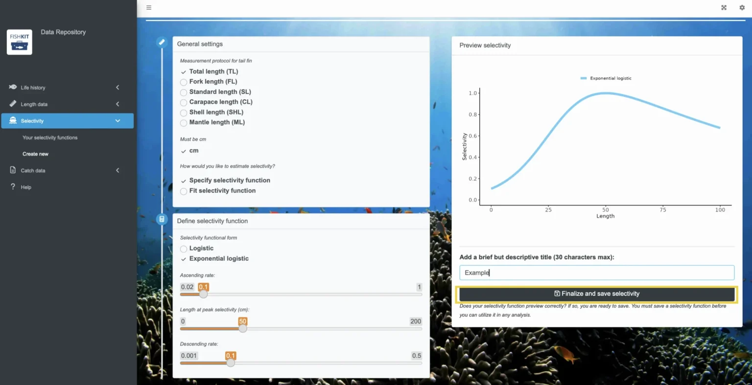
You should now be able to enter in information about your selectivity function. Start in the upper left box and enter in general settings information.
Enter in the measurement protocol for the tail fin, and note it must be in centimeters. Also note that this protocol should align with the length type for the life history you will be using in the Size Limit Builder.
Then, you have the option to specify the selectivity function parameters or fit the selectivity function. Specifying the parameters is the more typical approach, perhaps based on values obtained from an estimate made outside of FishKit.
Fitting the selectivity function occurs by inputting length-selectivity pairs, plotting the results, and fitting the function. This second approach may be most suitable when experts recognize an apparent selectivity pattern in the fishery but can only approximate its shape.
Relevant Modules:
D. Define the selectivity function
Scroll down to the second box in the left hand column. Here you will define the selectivity function. Note that as you enter in parameters, the corresponding graph on the right will automatically update.
If you selected “Specify selectivity function” in the previous step, start by selecting either logistic or exponential logistic as the function form. Then, drag the sliders for each parameter to the correct value. For a logistic form, you will specify the length at 50% selection and the increment to 95% selection. For an exponential logistic form, you will specify ascending rate, length at peak selectivity, and the descending rate.
Fitting to a sketch provides estimates of both logistic and exponential logistic function, and the user must select one function to save. The maximum likelihood fitting process requires starting values for parameter estimates as well as reasonable parameter bounds. For the logistic selectivity function, the starting value for the length at 50% selection (SL50) is the length at which selectivity is closest to 0.5 from the input data points. The starting value for the length at 95% selection (SL95) is the length at which selectivity is closest to 0.95 from the input data points. For the exponential logistic selectivity function, the starting values for the ascending rate (p1) and descending rate (p3) are set at 0.1 and 0.2 respectively. The starting value for the length at peak selectivity (p2) is the length at which the maximum selectivity occurs from the input data points. For the logistic selectivity function, the minimum value for SL50 is the minimum length represented in the input data set minus 20% (or 0 cm, whichever is higher) and the maximum value for SL50 is the maximum length represented in the input data set plus 20% (or 299 cm, whichever is less). The minimum and maximum values for SL95 are both 1 cm greater than the minimum and maximum values for SL50. For the exponential logistic selectivity function, p1 must be between 0.02 and 1, and p3 between 0.005 and 0.6. The minimum value for p2 is the minimum length represented in the input data set minus 20% (or 0 cm, whichever is higher) and the maximum value for p2 is the maximum length represented in the input data set plus 20% (or 300 cm, whichever is less).
Diagnostics are provided to aid you in selecting a suitable selectivity function to correspond with their sketch. Root-mean-square is provided as a measure of fit to the data, with lower values indicating a better fit. However, users should also consider parsimony in that the logistic function has fewer parameters and is interpreted as representing asymptotic selectivity. The exponential logistic has three parameters and can represent doming or right-hand selectivity but can also approximate asymptotic selectivity. Thus, if the fishing gear is expected to have asymptotic selectivity, the logistic function may be the better choice. An additional diagnostic is provided in the form of jitter analysis. The starting values for the five parameters are jittered 10 times within the parameter bounds prior to fitting the two selectivity functions to see if the same parameter estimates were returned. This is done to assess whether the absolute minima was likely found, or whether the fitting algorithm found a local minima. In cases where the absolute minima was unlikely to be found, parameter estimates are likely to vary between jitter runs. Where the jittered fit diagnostic displays orange boxes, these boxes indicate that that parameter estimate differs from the initial fit by more than 10%. Orange or red boxes indicate fitting problems. Additionally red boxes are displayed when a parameter has approached its bounds. It is advisable to discard a given function type for if orange or red boxes occur.
Relevant Modules:
E. Finalize and save selectivity function
Once you have entered in the parameters and your selectivity function previews correctly, you are ready to save. Start by entering a title in the box below the graph, and then click “Finalize and save selectivity.”
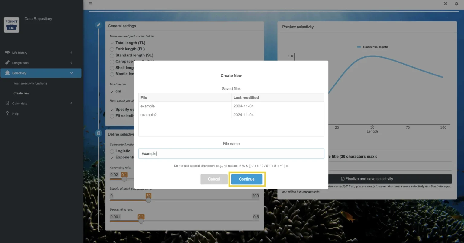
Re-enter your title without any spaces or special characters, and click “Continue.”
Click “Continue” again to save the file.
Relevant Modules:
F. View your selectivity function(s) (optional)
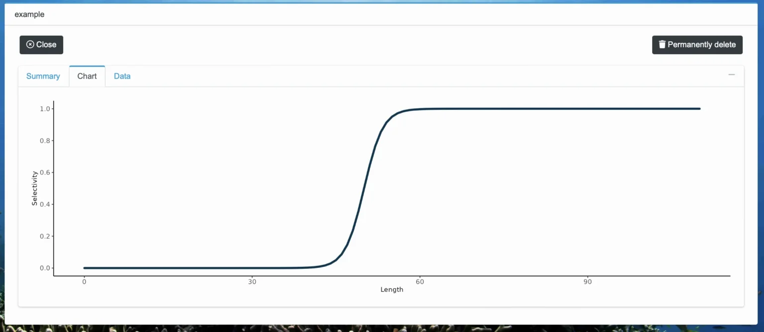
To view the selectivity function you just created, or to access your previous selectivity functions, click “Selectivity” and then “Your selectivity functions” from the dropdown menu.
Then, use the dropdown menu on the main page to choose the selectivity function you want to look at. Click on your desired function, and then click “Select.”
You will now see a box with three tabs, a “Summary” tab containing basic metadata information for your function, a “Chart” tab visualizing the function, and a “Data” tab that contains any associated data.
To close the selectivity function and look at a different one, click the “Close” button in the left corner.
Relevant Modules:


